The Assignment Problem
There are \(n\) people available to carry out \(n\) jobs. Each person is assigned to carry out exactly one job. Some individuals are better suited to particular jobs than others, so there is an estimated cost \(c_{ij}\) if person \(i\) is assigned to job \(j\). The problem is to find a minimum cost assignment.
Model
Definition of the variables.
\(x_ij = 1\) if person \(i\) does job \(j\), and \(x_{ij} = 0\) otherwise.
Definition of the constraints.
Each person \(i\) does one job:
\[ \sum_{j=1}^n x_{ij} =1 \text{ for \$i = 1,…, n\$} \]
Each job \(j\) is done by one person:
\[ \sum_{i=1}^n x_{ij} =1 \text{ for \$j = 1,…, n\$} \]
The variables are \(0–1\):
\[ x_{ij} ∈ \{0, 1\} \text{ for \$i = 1,…, n, j = 1,…, n\$} \]
Definition of the objective function.
The cost of the assignment is minimized:
\[ \min \sum_{i=1}^n \sum_{j=1}^n c_{ij}x_{ij} \]
Example
In the example there are five workers (numbered 0-4) and four tasks (numbered 0-3). Note that there is one more worker than in the example in the Overview.
The costs of assigning workers to tasks are shown in the following table.
| 0 | 1 | 2 | 3 | |
|---|---|---|---|---|
| 0 | 90 | 80 | 75 | 70 |
| 1 | 35 | 85 | 55 | 65 |
| 2 | 125 | 95 | 90 | 95 |
| 3 | 45 | 110 | 95 | 115 |
| 4 | 50 | 100 | 90 | 100 |
The problem is to assign each worker to at most one task, with no two workers performing the same task, while minimizing the total cost. Since there are more workers than tasks, one worker will not be assigned a task.
Solution using Gurobipy
Using the code below we get the following
Total cost = \(265.0\)
Worker \(0\) assigned to task \(3\). Cost = \(70\).
Worker \(1\) assigned to task \(2\). Cost = \(55\).
Worker \(2\) assigned to task \(1\). Cost = \(95\).
Worker \(3\) assigned to task \(0\). Cost = \(45\).
import gurobipy as gp
from gurobipy import GRB

costs = [
    [90, 80, 75, 70],
    [35, 85, 55, 65],
    [125, 95, 90, 95],
    [45, 110, 95, 115],
    [50, 100, 90, 100],
]

num_workers = len(costs)
num_tasks = len(costs[0])

m = gp.Model('GC')
x = m.addVars([(i,j) for i in range(num_workers) for j in range(num_tasks)], vtype = GRB.BINARY, name="assignment")

m.addConstrs((sum([x[(i,j)] for j in range(num_tasks)]) <= 1 for i in range(num_workers)))

m.addConstrs((sum([x[(i,j)] for j in range(num_workers)]) == 1 for j in range(num_tasks)))

m.setObjective(sum(costs[i][j] * x[(i, j)] for j in range(num_tasks) i in range(num_workers)), GRB.MINIMIZE)

m.optimize()

for v in m.getVars():
    if v.x:
        print(v.varName, v.x)
Here is the output from Gurobi
Gurobi Optimizer version 9.1.2 build v9.1.2rc0 (win64)
Thread count: 6 physical cores, 12 logical processors, using up to 12 threads
Optimize a model with 9 rows, 20 columns and 40 nonzeros
Model fingerprint: 0xd44ba4c8
Variable types: 0 continuous, 20 integer (20 binary)
Coefficient statistics:
  Matrix range     [1e+00, 1e+00]
  Objective range  [4e+01, 1e+02]
  Bounds range     [1e+00, 1e+00]
  RHS range        [1e+00, 1e+00]
Found heuristic solution: objective 385.0000000
Presolve time: 0.00s
Presolved: 9 rows, 20 columns, 40 nonzeros
Variable types: 0 continuous, 20 integer (20 binary)

Root relaxation: objective 2.650000e+02, 7 iterations, 0.00 seconds

    Nodes    |    Current Node    |     Objective Bounds      |     Work
 Expl Unexpl |  Obj  Depth IntInf | Incumbent    BestBd   Gap | It/Node Time

*    0     0               0     265.0000000  265.00000  0.00%     -    0s

Explored 0 nodes (7 simplex iterations) in 0.03 seconds
Thread count was 12 (of 12 available processors)

Solution count 2: 265 385

Optimal solution found (tolerance 1.00e-04)
Best objective 2.650000000000e+02, best bound 2.650000000000e+02, gap 0.0000%
assignment[0,3] 1.0
assignment[1,2] 1.0
assignment[2,1] 1.0
assignment[3,0] 1.0
Total Cost: 265.0
Graph Coloring
Graph coloring belongs to the classical optimization problems and has been studied for a long time. We consider the vertex coloring problem in which colors are assigned to the vertices of a graph such that no two adjacent vertices get the same color and the number of colors is minimized. The minimum number of colors needed for a given graph is called its \(\textbf{chromatic number}\) and denoted by \(χ\). Computing the chromatic number of a graph is NP-hard.Graph coloring problem has many applications, e.g., register allocation, scheduling, frequency assignment and timetabling etc.
Model
The classical ILP model for a graph \(G = (V, E)\) is based on assigning color \(i\) to vertex \(v ∈ V\). For this, it introduces assignment variables \(x_{vi}\) for each vertex \(v\) and color \(i (i = 1, . . . , H)\), with \(x_{vi} = 1\) if vertex \(v\) is assigned to color \(i\) and \(x_{vi} = 0\) otherwise. \(H\) is an upper bound of the number of colors (e.g., the result of a heuristic) and is at most \(|V|\). For modelling the objective function, additional binary variables \(w_i\) are needed which get value \(1\) if and only if color \(i\) is used in the coloring \((i = 1, . . . , H)\). The model is given by:
\[ \begin{align} &\underset{1 \leq i \leq H}{\min} \sum w_i \\\\ \text{s.t.} & \sum_{i=1}^H x_{vi} = 1 \text{ $\forall v \in V$} \\\\ & x_{ui} + x_{vi} \leq w_i \text{ $\forall (u,v) \in E, i = 1, \dots, H$} \\\\ &x_{vi}, w_i \in \{0,1\} \text{ $\forall v \in V, i = 1, \dots, H$} \end{align} \]
The objective function minimizes the number of used colors. Equation \((2)\) ensures that each vertex receives exactly one color. For each edge there is a constraint \((3)\) making sure that adjacent vertices receive different colors. This model has the advantage that it is simple and easy to use. It can be easily extended to generalizations and/or restricted variants of the graph coloring problem. Since the number of variables is quadratic in \(|V|\) (it is bounded by \(H(|V| + 1))\) and the number of constraints is cubic in \(|V|\) (exactly \(|V| + H|E| = O(|V||E|)\) constraints of type \(2\) and \(3\)), it can directly be used as input for a standard ILP solver.
Example
Given is set of \(n\) people, \(S = \{s_1, s_2, \dots, s_n\}\), and the task is to group them. However, people who have conflicts between each other cannot be assigned to the same group. Let graph \(G = (E, S)\) represent this scenario. Edges of this graph represent conflicts. Figure below illustrates a sample scenario. Note that any two people who are connected by an edge are not assigned the same group. Formulate this as an integer programming problem. 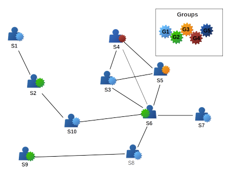
Solution using Gurobipy
Using the code below we see that only \(3\) colours are required to color the graph. The coloring is shown below 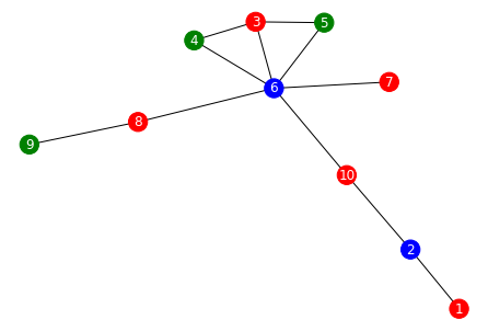
import gurobipy as gp
from gurobipy import GRB
from itertools import product

# list of vertices
V = list(range(1,11))

# list of edges
E = [(1,2),(2,10),(9,8),(10,6),(8,6),(3,6),(3,4),(4,6),(5,6),(3,5),(6,7)]

# create the model
m = gp.Model('GC')

# declare variables for colors used
w = m.addVars(V, vtype = GRB.BINARY, name="colors")

# declare variables for vertex colors
x = m.addVars(list(product(V,V)), vtype=GRB.BINARY, name="vertex_colors")

# constraint - one color per vertex
m.addConstrs((sum([x[(v,i)] for i in V])==1 for v in V), name='one_vertex_color')

# constraint - different colors for vertices connected by an edge
m.addConstrs((x[(u,i)] + x[(v,i)] <= w[i] for (u,v) in E for i in V), name='edge_diff_color')

# objective - minimizing the number of colors used
m.setObjective(sum(w[i] for i in V), GRB.MINIMIZE)

m.optimize()

# printing the values of decision variables
for v in m.getVars():
    if v.x:
        print(v.varName, v.x)
Here is the output from Gurobi
Gurobi Optimizer version 9.1.2 build v9.1.2rc0 (win64)
Thread count: 6 physical cores, 12 logical processors, using up to 12 threads
Optimize a model with 120 rows, 110 columns and 430 nonzeros
Model fingerprint: 0x65c24c79
Variable types: 0 continuous, 110 integer (110 binary)
Coefficient statistics:
  Matrix range     [1e+00, 1e+00]
  Objective range  [1e+00, 1e+00]
  Bounds range     [1e+00, 1e+00]
  RHS range        [1e+00, 1e+00]
Found heuristic solution: objective 6.0000000
Presolve removed 30 rows and 0 columns
Presolve time: 0.00s
Presolved: 90 rows, 110 columns, 360 nonzeros
Variable types: 0 continuous, 110 integer (110 binary)

Root relaxation: objective 3.000000e+00, 53 iterations, 0.00 seconds

    Nodes    |    Current Node    |     Objective Bounds      |     Work
 Expl Unexpl |  Obj  Depth IntInf | Incumbent    BestBd   Gap | It/Node Time

*    0     0               0       3.0000000    3.00000  0.00%     -    0s

Explored 0 nodes (53 simplex iterations) in 0.03 seconds
Thread count was 12 (of 12 available processors)

Solution count 2: 3 6

Optimal solution found (tolerance 1.00e-04)
Best objective 3.000000000000e+00, best bound 3.000000000000e+00, gap 0.0000%
colors[1] 1.0
colors[4] 1.0
colors[5] 1.0
vertex_colors[1,1] 1.0
vertex_colors[2,4] 1.0
vertex_colors[3,1] 1.0
vertex_colors[4,5] 1.0
vertex_colors[5,5] 1.0
vertex_colors[6,4] 1.0
vertex_colors[7,1] 1.0
vertex_colors[8,1] 1.0
vertex_colors[9,5] 1.0
vertex_colors[10,1] 1.0
The \(0–1\) Knapsack Problem
There is a budget \(b\) available for investment in projects during the coming year and \(n\) projects are under consideration, where \(a_j\) is the outlay for project \(j\) and \(c_j\) is its expected return. The goal is to choose a set of projects so that the budget is not exceeded and the expected return is maximized.
Model
Definition of the variables.
\(x_j = 1\) if project \(j\) is selected, and \(x_j = 0\) otherwise.
Definition of the constraints.
The budget cannot be exceeded:
$ _{j=1}^n a_j x_j ≤ b$.
The variables are \(0–1\):
$x_j {0, 1} $
Definition of the objective function.
The expected return is maximized:
\(\max \sum_{j=1}^n c_j x_j\).
Example
You are given a knapsack of \(16\) units capacity and a set of \(5\) items. Each item is represented by the tuple of the form (item number, value, weight). The following are the items: \((1,5,4), (2,6,2), (3,2,6), (4,5,8), (5,3,5)\). Identify the highest valued sub-collection of items that can be fit inside the knapsack.
Solution using Gurobipy
Using the code below, we see that items \(1\), \(2\) and \(4\) need to be selected for a maximum value of \(16\).
import gurobipy as gp
from gurobipy import GRB

items = [(1,5,4), (2,6,2), (3,2,6), (4,5,8), (5,3,5)]

m = gp.Model('KS')
x = m.addVars([i for i,_,_ in items], vtype = GRB.BINARY, name="selected")
m.addConstr(sum(x[i]*w for (i,_,w) in items) <= 16, name='weight')
m.setObjective(sum(x[i]*v for i,v,_ in items), GRB.MAXIMIZE)
m.optimize()

for v in m.getVars():
    if v.x:
        print(v.varName, v.x)

print(f'Total Value: {m.objVal}')
Here is the output from Gurobi
Gurobi Optimizer version 9.1.2 build v9.1.2rc0 (win64)
Thread count: 6 physical cores, 12 logical processors, using up to 12 threads
Optimize a model with 1 rows, 5 columns and 5 nonzeros
Model fingerprint: 0xad9237f2
Variable types: 0 continuous, 5 integer (5 binary)
Coefficient statistics:
  Matrix range     [2e+00, 8e+00]
  Objective range  [2e+00, 6e+00]
  Bounds range     [1e+00, 1e+00]
  RHS range        [2e+01, 2e+01]
Found heuristic solution: objective 13.0000000
Presolve removed 1 rows and 5 columns
Presolve time: 0.00s
Presolve: All rows and columns removed

Explored 0 nodes (0 simplex iterations) in 0.02 seconds
Thread count was 1 (of 12 available processors)

Solution count 2: 16 13

Optimal solution found (tolerance 1.00e-04)
Best objective 1.600000000000e+01, best bound 1.600000000000e+01, gap 0.0000%
selected[1] 1.0
selected[2] 1.0
selected[4] 1.0
Total Value: 16.0
The Set Covering Problem
Given a certain number of regions, the problem is to decide where to install a set of emergency service centers. For each possible center, the cost of installing a service center and which regions it can service are known. For instance, if the centers are fire stations, a station can service those regions for which a fire engine is guaranteed to arrive on the scene of a fire within eight minutes. The goal is to choose a minimum cost set of service centers so that each region is covered. Let \(M = \{1,…,m\}\) be the set of regions, and \(N = \{1,…, n\}\) the set of potential centers. Let \(S_j ⊆ M\) be the regions that can be serviced by a center at \(j ∈ N\) and \(c_j\) its installation cost. We obtain the problem:
\[ \underset{T \subseteq N}{\min} \left\\{ \sum_{j \in T} c_j ∶ \cup_{j \in T} S_j = M \right\\} \]
Model
To facilitate the description, we first construct a \(0–1\) incidence matrix \(A\) such that \(a_{ij} = 1\) if \(i ∈ S_j\) and \(a_{ij} = 0\), otherwise.
Definition of the variables.
\(x_j = 1\) if center \(j\) is selected, and \(x_j\) = 0 otherwise.
Definition of the constraints.
At least one center must service region \(i\):
\(\sum_{j=1}^n a_{ij}x_j ≥ 1 \text{ for \$i = 1,…,m\$}\).
The variables are \(0–1\):
\(x_j ∈ \{0, 1\} \text{ for \$j = 1,…, n\$}\).
Definition of the objective function.
The total cost is minimized:
\(\min \sum_{j=1}^n c_j x_j\).
Example
Let’s consider a simple example where we assign cameras at different locations. Each location covers some areas of stadiums, and our goal is to put the least amount of cameras such that all areas of stadiums are covered. We have stadium areas from \(1\) to \(15\), and possible camera locations from \(1\) to \(8\).
The stadium areas that the cameras can cover are given in table below:
| Camera Location | 1 | 2 | 3 | 4 | 5 | 6 | 7 | 8 |
|---|---|---|---|---|---|---|---|---|
| Stadium Area | 1,3,4,6,7 | 4,7,8,12 | 2,5,9,11,13 | 1,2,14,15 | 3,6,10,12,14 | 8,14,15 | 1,2,6,11 | 1,2,4,6,8,12 |
Here \(M=\{1, \dots, 15\}\) and \(N=\{1, \dots, 8\}\).
We can then represent the above information using binary values. If the stadium area \(i\) can be covered with camera location \(j\), then we have \(a_{ij}=1\). If not,\(a_{ij}=0\). For instance, stadium area \(1\) is covered by camera location \(1\), so \(a_{11}=1\), while stadium area \(1\) is not covered by camera location \(2\), so \(a_{12}=0\). The binary variables \(a _{ij}\) values are given in the table below:
| Camera1 | Camera2 | Camera3 | Camera4 | Camera5 | Camera6 | Camera7 | Camera8 | |
|---|---|---|---|---|---|---|---|---|
| Stadium1 | 1 | 1 | 1 | 1 | ||||
| Stadium2 | 1 | 1 | 1 | 1 | ||||
| Stadium3 | 1 | 1 | ||||||
| Stadium4 | 1 | 1 | 1 | |||||
| Stadium5 | 1 | |||||||
| Stadium6 | 1 | 1 | 1 | 1 | ||||
| Stadium7 | 1 | 1 | ||||||
| Stadium8 | 1 | 1 | 1 | |||||
| Stadium9 | 1 | |||||||
| Stadium10 | 1 | |||||||
| Stadium11 | 1 | 1 | ||||||
| Stadium12 | 1 | 1 | 1 | |||||
| Stadium13 | 1 | |||||||
| Stadium14 | 1 | 1 | 1 | |||||
| Stadium15 | 1 | 1 |
We introduce the binary variable \(x_{j}\) to indicate if a camera is installed at location \(j\). \(x_{j}=1\) if camera is installed at location \(j\), while \(x_{j}=0\) if not.
Our objective now is to minimize \(\min \sum_{j=1}^8 x_j\)
subject to the constraints \(\sum_{j=1}^8 a_{ij}x_j ≥ 1 \text{ for \$i = 1,…,15\$}\).
Solution using Gurobipy
Using the code below, we see that at a minimum \(4\) cameras(e.g. \(2\), \(3\), \(4\) and \(5\)) are required.
import gurobipy as gp
from gurobipy import GRB

a = [[1,0,0,1,0,0,1,1],
     [0,0,1,1,0,0,1,1],
     [1,0,0,0,1,0,0,0],
     [1,1,0,0,0,0,0,1],
     [0,0,1,0,0,0,0,0],
     [1,0,0,0,1,0,1,1],
     [1,1,0,0,0,0,0,0],
     [0,1,0,0,0,1,0,1],
     [0,0,1,0,0,0,0,0],
     [0,0,0,0,1,0,0,0],
     [0,0,1,0,0,0,1,0],
     [0,1,0,0,1,0,0,1],
     [0,0,1,0,0,0,0,0],
     [0,0,0,1,1,1,0,0],
     [0,0,0,1,0,1,0,0]]

n_cams, n_stads = 8, 15
m = gp.Model('SC')
x = m.addVars(list(range(1, n_cams+1)), vtype = GRB.BINARY, name="camera")
m.addConstrs((sum(a[i][j]*x[j+1] for j in range(n_cams)) >=1 for i in range(n_stads)),
name='stadium_coverage')
m.setObjective(sum(x[i+1] for i in range(n_cams)), GRB.MINIMIZE)
m.optimize()

for v in m.getVars():
    if v.x:
        print(v.varName, v.x)

print(f'Total Value: {m.objVal}')
Here is the output from Gurobi
Gurobi Optimizer version 9.1.2 build v9.1.2rc0 (win64)
Thread count: 6 physical cores, 12 logical processors, using up to 12 threads
Optimize a model with 15 rows, 8 columns and 36 nonzeros
Model fingerprint: 0x098bdca7
Variable types: 0 continuous, 8 integer (8 binary)
Coefficient statistics:
  Matrix range     [1e+00, 1e+00]
  Objective range  [1e+00, 1e+00]
  Bounds range     [1e+00, 1e+00]
  RHS range        [1e+00, 1e+00]
Found heuristic solution: objective 5.0000000
Presolve removed 11 rows and 3 columns
Presolve time: 0.00s
Presolved: 4 rows, 5 columns, 10 nonzeros
Variable types: 0 continuous, 5 integer (5 binary)

Root relaxation: objective 4.000000e+00, 4 iterations, 0.00 seconds

    Nodes    |    Current Node    |     Objective Bounds      |     Work
 Expl Unexpl |  Obj  Depth IntInf | Incumbent    BestBd   Gap | It/Node Time

*    0     0               0       4.0000000    4.00000  0.00%     -    0s

Explored 0 nodes (4 simplex iterations) in 0.03 seconds
Thread count was 12 (of 12 available processors)

Solution count 2: 4 5

Optimal solution found (tolerance 1.00e-04)
Best objective 4.000000000000e+00, best bound 4.000000000000e+00, gap 0.0000%
camera[2] 1.0
camera[3] 1.0
camera[4] 1.0
camera[5] 1.0
Total Value: 4.0
Example - class scheduling
John Dupont is attending a summer school where he must take four courses per day. Each course lasts an hour, but because of the large number of students, each course is repeated several times per day by different teachers. Section \(i\) of course \(k\) denoted \((i, k)\) meets at the hour \(t_{ik}\), where courses start on the hour between \(10\) a.m. and \(7\) p.m. John’s preferences for when he takes courses are influenced by the reputation of the teacher, and also the time of day. Let \(p_{ik}\) be his preference for section \((i, k)\).Unfortunately, due to conflicts, John cannot always choose the sections he prefers.
Formulate an integer programto choose a feasible course schedule that maximizes the sum of John’s preferences.
Modify the formulation so that John never has more than two consecutive hours of classes without a break.
Modify the formulation so that John chooses a schedule in which he starts his day as late as possible.
Model
Let the number of courses be \(c\), the maximum number of sections per course be \(s\) and let the number of time periods in a day be \(p\).
Part (i)
Input.
Let \(a_{ijk}=1\) if \(i = t_{kj}\), i.e. there is a class of course \(j\) for section \(k\) at time \(i\) or \(a_{ijk}=0\) otherwise.
Definition of the variables.
\(x_{ijk} = 1\) if section \(k\) of course \(j\) is selected at time period \(i\) and \(x_{ijk} = 0\) otherwise.
Definition of the constraints.
At most one class can be taken in a given time period. \(\sum_{j,k} a_{ijk} \cdot x_{ijk} \leq 1\) where \(i \in \{1, \dots,p\}\), \(j \in \{1, \dots,c\}\) and \(k \in \{1, \dots,s\}\).
At most one section can be taken per course in a day. \(\sum_{i,j} a_{ijk} \cdot x_{ijk} \leq 1\) where \(i \in \{1, \dots,p\}\), \(j \in \{1, \dots,c\}\) and \(k \in \{1, \dots,s\}\).
Four courses must be taken in a day. \(\sum_{i,j,k} a_{ijk} \cdot x_{ijk} = 4\) where \(i \in \{1, \dots,p\}\), \(j \in \{1, \dots,c\}\) and \(k \in \{1, \dots,s\}\).
Definition of the objective function.
The sum of preferences should be maximized:
\(\max \sum_{i} a_{ijk} \cdot x_{ijk} \cdot p_{kj}\) where \(i \in \{1, \dots,p\}\), \(j \in \{1, \dots,c\}\) and \(k \in \{1, \dots,s\}\).
Part (ii)
If John can never have more than two consecutive hours of classes, he cannot take more than two classes in any three consecutive time periods. We need the following addtional constraint:
\(\sum_{i,j,k} a_{ijk} \cdot x_{ijk} + a_{(i+1)jk} \cdot x_{(i+1)jk} + a_{(i+2)jk} \cdot x_{(i+2)jk} \leq 2\) where \(i \in \{1, \dots,p-2\}\), \(j \in \{1, \dots,c\}\) and \(k \in \{1, \dots,s\}\).
Part (iii)
If John chooses a schedule where he starts his day as late as possible, this is equivalent to maximizing the sum of the starting times. The objective function should be modified as follows:
\(\max \sum_{i} i \cdot a_{ijk} \cdot x_{ijk}\) where \(i \in \{1, \dots,p\}\), \(j \in \{1, \dots,c\}\) and \(k \in \{1, \dots,s\}\).